3.2 Basic Examples

3.2.1 Inline Commands

For inline sage commands, use \sage{}. For example, $\sage{diff(x^3, x, 2)}$ prints \(6x\), the second derivative of \(x^3\).

3.2.2 Blocks

• To execute and print a block of sage commands, use the sageblock environment. For example,

\begin{sageblock}
    f(x) = exp(x) * sin(2*x)
\end{sageblock}

• To execute and hide a block of sage commands, use the sagesilent environment. For example,

\begin{sagesilent}
    f(x) = exp(x) * sin(2*x)
\end{sagesilent}

• To print only psuedo-codes, use the sageverbatim environment. For example,

\begin{sageverbatim}
    f(x) = exp(x) * sin(2*x)
\end{sageverbatim}

3.2.3 Graphics

To add graphs, use \sageplot[options]{2D or 3D plot commands}. (Although the example shown here is a 2D graph, 3D graphs work in the same way. Here are the SageMath guides for 2D graphics and 3D graphics.)

\begin{figure}[h]
\sageplot[width=0.5\textwidth]{plot(x^3, (x, -1, 1))}
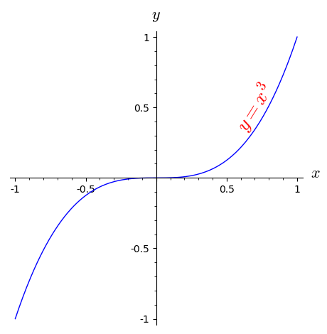
\end{figure}

For more delicated plots, use a sagesilent block to draw the graph, then call the graph in \sageplot. For example,

\begin{sagesilent}
a = plot(x^3, (x, -1, 1), axes_labels=['$x$', '$y$'], aspect_ratio=1);
a += text('$y=x^3$', (0.7, 0.5), rotation=58, fontsize='20', fontweight='bold', color='red')
\end{sagesilent}

\begin{figure}[h]
\sageplot[width=0.5\textwidth]{a}
\end{figure}